
My First Dive into Variant Calling
Variant calling is the process of identifying mutations and differences between a sample genome and a reference. In this post, I walk through my experience going from raw whole genome sequencing (WGS) reads all the way to visualizing variants in IGV. It was my first time running a full bioinformatic workflow on my own, so I’m excited to share what I learned—challenges, surprises, and all!
GENOMICSSTATISTICS
Sohum Bhardwaj
4/18/20259 min read
While I have coded some genomic algorithms from scratch like sequence alignment and de novo read assembly, I have never actually used popular genomics tools or performed analysis from an end-to-end workflow, going from sequenced reads to variant analysis. Now that I have time during spring break, I figured I would give it a shot!
My plan was simple: to take sequenced reads, assemble them, and then analyze the variance from the human genome. Along the way, I learned a lot more about bioinformatic workflows, got to see how sequence alignment is really awesome, and encountered my fair share of biological quirkiness!
But first, what exactly is the goal? What is variant calling?
As you probably know, almost all human genomes have some degree of variance in the form of genetic mutations. Analyzing these variants can lead to insights in population genetics, cancer, and is the foundation of many genomic fields.
However, to identify the genetic variants we need to sort through a lot of false positives produced by sequencing errors and lab errors. This process is what variant calling is about. But to even start variant calling, we need to assemble the sample genome from a bunch of read. And if you don't understand what that means, don't worry, I will explain the significance of every step as we go, so that by the end, you too will have an idea of what an end-to-end workflow looks like!
If you want to try it for yourself, here is the guide I followed to help me out: Worked Example | Introduction to Genomics for Engineers
Fair Warning: Be prepared to spend a couple hours in environment setup hell. Especially, if you are on windows since most likely you will have to setup WSL, or follow this guide.
Intro
Quality Checking Reads
What is in these FASTQ Files?
FASTQ files contain data about sequenced reads. They will have identification information, the raw sequence, and a quality score for each base.
I am using a pair of FASTQ files that represent paired-end reads. This means that of a large DNA fragment, the sequencer reads from each end a certain amount of base pairs. For example, if the DNA fragment was 10 bp, each paired-end read might be 4 bp.
AGTC ---- 2bp in between ---- TCAG
In reality we don't know the insert size, this means we have a raw sequence of 80 bp, and another raw sequence of 80 bp and we know that there is a certain amount of bases in between them, but we don’t know how many or what they might be.
How could this information be useful? You may be thinking. It seems like we have just a few puzzle pieces in a really big (billions of bases) puzzle. Wouldn’t it be easier to just read the entire fragment? Well, due to how the sequencing process works, as you go down a read, the quality score drops dramatically.
And, despite what it may seem, we can figure out how big the fragment was (the insert size), and what was between the two reads rather easily thanks to the availability of reference genomes–but I am getting ahead of myself.
But, first we need to check that these FASTQ files actually have stuff in them.
Generating the Report
Running this command uses the FASTQC tool to generate a report on the FASTQ file:
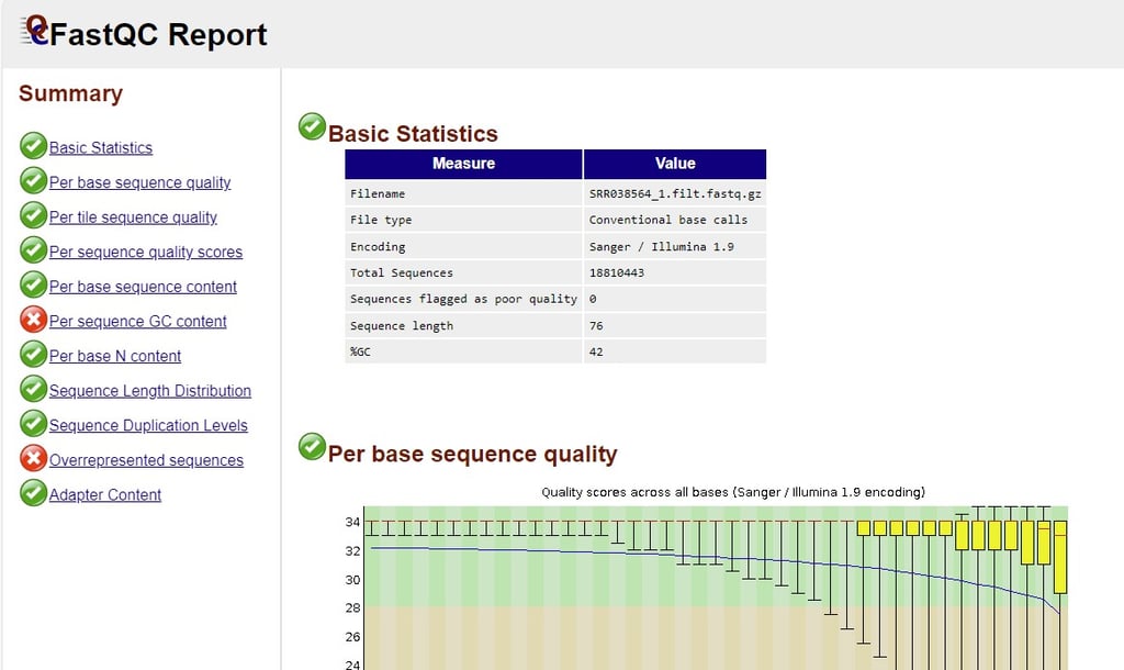
GC content
Initially I saw 42% and thought it seemed rather low and hypothesized that I might have messed up the file. Luckily a quick google search alleviated my fears, it turns out that the average GC content of the human genome is 41%, so I was right on target.
Confidence tapering off
I know I mentioned this above as well, but it was nice to see it confirmed in the FASTQ report. The confidence is clearing tapering off by the 70th base. It also was interesting to see that the reads were rather small, most of them being 76 bases.
Some observations
Indexing the Reference Genome
What is it a Reference Genome?
A reference genome is simply a genome constructed from a few humans. It isn’t necessarily the most common genome, as we will find out later. The human reference genome I am using is GRCh38, it stands for Genome Research Consortium human build 38–say that three times fast.
What does it mean to index one?
Well, I need the reference genome in order to align the reads contained in those FASTQ files. Alignment is simply finding where in the genome (3.8 billion base pairs) the reads match the most.
The problem is that the genome is 3.8 billion base pairs. That is so many bases that if we could read 20 of them a second–which is blazingly fast for a human–it would take over six years to finish reading. We need a better way to search for alignments considering we have hundreds of thousands of reads to align, luckily we can do something called indexing.
Think of an index in a book, it tells the reader what pages contain a specific keyword. An index for a genome is very similar. It contains the locations where we can find different subsequences in the genome.
One data structure that represents an index is a suffix array. For example, the suffix array entry for “AGCTGATGCTGAT” will have the coordinates of this sequence in the genome, if it exists. Suffix arrays get their name because they store all the suffixes of a sequence. So, for our example sequence, the suffix array would contain GCTGATGCTGAT, CTGATGCTGAT, TGATGCTGAT, etc. We create other data structures too, but they are beyond the scope of this post.
Running this command will create the several data structures that will help us align the sample genome to the reference faster:
There are some interesting products to this command:
This file specifies the ambiguous regions of the reference genome. In fact, when you open up the reference genome, it turns out the first few thousand bases are ambiguous. When I first saw the wall of N’s (N standing for ambiguous), I thought that my download was corrupted.
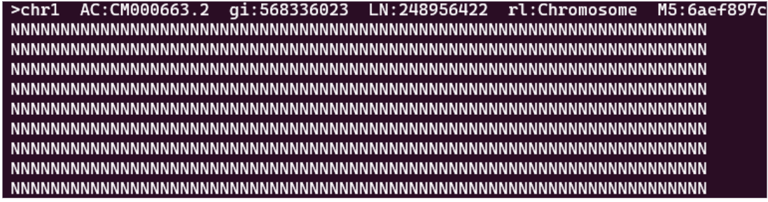
First couple hundred bases of the reference genome (N = ambiguous)
There are many reasons why there might be ambiguous regions in a genome. At the beginning of chromosomes there are telomeres. These repetitive sections of DNA protect the chromosome from damage. However, long repetitive stretches of DNA can be troublesome for alignment as reads may find alignments with several different sections. It is easier and more efficient to leave these regions ambiguous.
This is an annotation file for the genome. It specifies each region (contig) of the genome from chromosome 1 to unmarked regions.
You may notice that the annotation file specifies the mitochondrial genome as well!
Aligning the Reads
Aligning the reads is done with this command:
This creates a Sequence Alignment Map (.sam) file, we need to sort it and convert it into a Binary Alignment Map (.bam) file to get it ready for downstream analysis tools
This is slightly different from the guide since sorting a .sam directly was not working for me, but first converting it to a .bam worked.
By finding the coordinates (index in the reference genome) of each of the paired ends (aka alignment), we can now determine the insert size by measuring the distance between the start of the first read and the end of the second read. In reality, the fragments are a bit bigger than the insert size due to adapter sequences which are affixed to either end during sequencing.
Post-Processing
We first mark any duplicate reads. Duplicate reads arise mainly from PCR. Which is used to create multiple copies of the fragments so that the sequencer has a higher chance of sequencing them, but the duplicates can interfere with downstream analysis if they are left in.
For example, I am going to identify the point mutations (also called single nucleotide polymorphisms) in the alignment. Variant calling programs will use statistical models to determine how likely it is for a difference in the reference and the alignment to be a genuine biological variant.
Duplicates will make it seem like there is much more evidence that a variant exists than there is in reality.
We mark duplicates using a tool called picard:
Using another command we can check out our .bam file now
4.4 million duplicates were marked. That is a lot. If you are wondering what all the plus zeroes stand for. They represent the number of sequences that failed quality control checks. Since I have not set any in place, all the reads have passed–I am nothing but gracious :)
This command will first pileup all the reads in the alignment file, and then will calculate whether to call a variant or not, storing all the called variants in a .vcf (variant call format) file.
Visualizing with IGV
While we can use some shell commands to parse the VCF file, it is way more fun to use a visualization software such as IGV (Integrative Genomics Viewer).
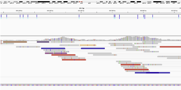
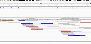
(I got a bit lucky here, most of the genome is not this colorful)
IGV can visualize reads that have been aligned to the reference genome. The colored genomes are discordant reads, or reads that map to different chromosomes, and This section of the genome has an awful lot of them.
Discordant can often be signs of chromosomal mutations if there is a buildup in a specific region. If a researcher was looking for a breakpoint (start of a chromosomal mutation), they may sequence this part of the genome again with a targeted sequencing because the coverage (aka number of reads overlapping a region) of this genome is rather low.
chromosomal mutations are often called structural variations in genomics
Only around 10x when 30x is recommended to reliably identified SNPs (single nucleotide polymorphisms/variations) and more is recommended to identify chromosomal mutations.
For fun I pulled up insertion or deletion calls with high confidence. I specified calls from only the autosomal and sex chromosomes, excluding anything in the mitochondrial genome.
On the left is the confidence of the variant measured on the Phred scale. A score of 200 has an astronomically low chance of being incorrect. Approximately a one in a hundred quintillion chance of being an error. Clearly, the program is very confident in these variants.
Let’s pull up the second one in IGV. AGT -> AGTGT
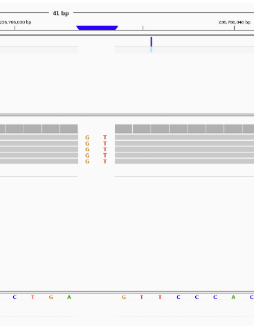
It shows us that all 5 reads found the INDEL which is probably why the program was so confident.
You may be wondering why I called it an INDEL instead of an insertion, the reason is that whether a mutation is an insertion or deletion is dependent on your perspective. It could have been an insertion of GT into the sample genome, but it could also have been a deletion of GT from the reference genome.
Lastly, I want to see the RS (Reference SNP) number of this mutation which will allow us to get some more information about it. In this workflow we did not annotate the .vcf file with the RS numbers so I will have to search the database for it.
There are definitely more efficient ways of doing it, but I decided to download the entire (28 GB) dbSNP database for hg38 (yea it took a while). The dbSNP database catalogues many common and rare SNPs in the human genome. Using it, we can query it for the mutation:
A quick inspection into the database reveals that the entries have special names for contigs (contiguous sequences, i.e. chromosomes):
Searching with this revised command reveals the rs number:
Along with a lot of other information that we will also find in the online database in a more human-friendly format. Check out the entry for yourself here.
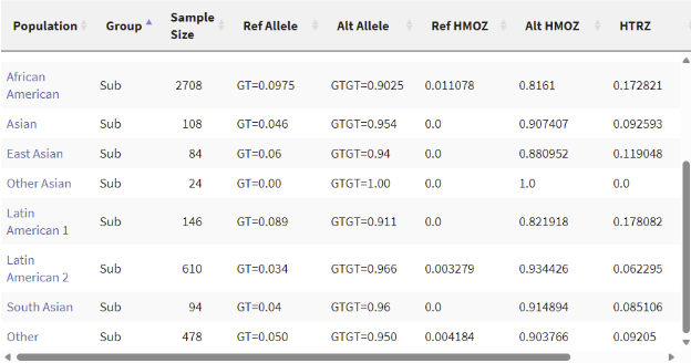
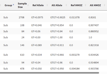
It seems that this mutation isn’t rare at all. It has over a 90% chance of appearing in all of the populations measured, in fact, not having this mutation is rather rare. To be honest, I am a little disappointed that the mutation wasn’t very special, but it makes sense considering I simply selected a random INDEL with high confidence.
Conclusion
Through this workflow, we went from a pair of FASTQ reads to being able to identify the genomic variations in the sample. In the future, I don’t think I am going to align the reads locally if I can help it–it takes a ridiculously long time! However, I will definitely revisit this again and try to analyze a much larger sample.