Why Single Cell Data Sucks (and How Bioinformaticians Cleanse It)

What and Why Single Cell Molecular Profiling

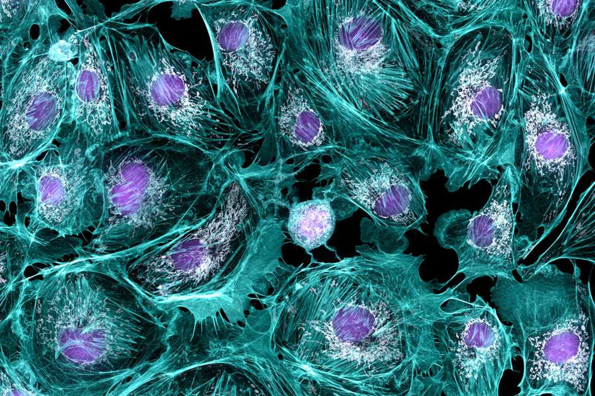
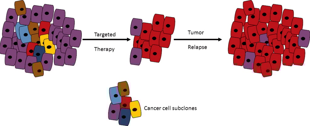
Single cell molecular profiling are technologies that capture the molecular profile of an entire cell together. For example, scRNA-seq assays allow for the sequences of the "entire" transcriptome of a cell for analysis (you will see why I put "entire" in quotation marks soon). This is useful because cells contain tens of thousands of expressed genes at any given time. scRNA-seq techniques allow researchers to gain a snapshot of the cell's gene expression which was not possible with previous bulk sequencing techniques. This is an incredibly powerful technique for capturing something called cell heterogeneity. Cell heterogeneity is the variation of cells within a population. If I took the cells from your blood, per say, each blood cell would have its own unique protein and gene expression. This may sound very obvious, of course all cells are not the same! But the implications are profound. Let's look at a specific example of tumor heterogeneity, or more specifically intratumor heterogeneity. When cells are taken from a tumor via biopsy, there is always a chance that some variations of cells may not be captured by the biopsy. This can lead to the incorrect treatment being prescribed leads to the tumor relapsing and even developing drug resistance. Single cell technologies can help researcher study tumors because they offer unparalleled detail into the state of the cell and its changes in genomic expression. They also offer keys to several other areas like trajectory influence, differentiation analysis, and provide the ability to form new novel hypotheses. For this blog post I will focus on scRNA-seq data because it is easy to think about this form of data compared to other modalities (types of data).

Single Cell Data Processing: The Lab Stage

This image shows an example of a therapy that targeted the brown, blue, and yellow variants of this tumor very well but was not able to target the red variant tumor leading to relapse. Tumor heterogeneity can have dangerous implications

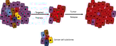
Before single cell data can be analyzed, it has to be procured, duh! This laboratory process begins with single cell sorting. During this stage, the cells are separated and surrounded by droplets via specialized techniques. These droplets contain various enzymes that break down the cell membrane and extract the mRNA which is converted in cDNA, complementary DNA, for sequencing. During this process, barcodes are attached to the mRNA to identify which cell the mRNA came from, and UMIs (universal molecular identifiers) are also attached to uniquely mark each molecule of mRNA. These barcodes and UMIs take the form of nucleotide sequences affixed to the end of the mRNA and are used in data processing stages to identify duplicate mRNA as well as group sequenced genes by cell. After the droplets do their work, the cDNA is amplified by PCR which creates many copies of the DNA. PCR is necessary to avoid drop out effects which is when a certain gene is not sequenced even though it is expressed in the cell. It is important to note that the UMIs attached to the mRNAs (which are transcribed onto the cDNA) are used to identify duplicates that arise from the PCR process, we only want each mRNA molecule to be represented once in our data. After PCR amplification, sequencing occurs. Sequencing can be a stochastic, random, process this means that sometimes cDNAs are not read by the sequencing machine which is partially mitigated by the previous amplification step. This is why I put "entire" in quotation marks: there is no guarantee that all of the transcriptome is sequenced. By the end of sequencing we have a bunch of messy mRNA reads that should represent the transcriptome of every cell that we have sequenced. A quick disclaimer: I have greatly simplified this process which is extremely complex and requires using a variety of novel biotechnologies. Many inconsistencies with the data such as batch effects, drop out effects, doublets, and mRNA leaks that arise from this step must be corrected through computational algorithms during data preprocessing.

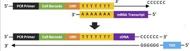
This image shows how the mRNA transcript is transformed into a cDNA with a cell barcode and UMI. (Image credits and further reading)

Quality Control - The First Step

Quality Control is the first step of data preprocessing which is what the remainder of this post will cover. Data preprocessing is used in a variety of data fields and involves cleaning up the data and removing biases which may impact further analysis as well as the simplifying and summarization of the data. The first step, Quality control, involves getting rid of outliers and bad data. In quality control, three main covariates are used to filter out this bad data (see below).
Quick note, instead of per cell it is practice to refer to these metrics per barcode because sometimes multiple cells are encapsulated in the same droplet and therefore have the same barcode, aka a doublet. Or, oftentimes, a droplet does not encapsulate any cells at all so the barcode is "empty" (in reality there are some genes from these barcodes due to ambient gene expression which happens when broken cells and contaminate the suspension).

Counts per Barcode (aka Count Depth)
A count is recorded each time a sequencing machine reads a unique cDNA molecule. Count depth is simply the number of mRNA transcripts that were inside the cell.

Genes per Barcode
One gene or one mRNA can have multiple counts. The genes per barcode illustrates how many unique genes were present in the barcode.

Fraction of counts from Mitochondrial genes per Barcode
Some counts come from genes that were within the mitochondria. The amount of the counts that come from mitochondrial genes rather than genes from the DNA can indicate certain errors.

These covariates are used to determine errors. For example a barcode with high count depth and a high amount of detected genes is likely a doublet. Similarly, a barcode with a low count debt, low amount of detected genes, but high fraction of mitochondrial genes is indicative of a broken cell whose cytoplasmic mRNA leaked out. Thresholds are placed based on these covariates which filters out data points which are likely problematic.
Ambient gene expression can also be filtered out by looking at data from those "empty" barcodes though not all quality control procedures involve this step. Quality control plays an important step to account for certain lab errors but more complex errors like batch effects require more powerful methods.

Normalization

Biological data has a lot of inherent randomness and laboratory procedures add a lot more. Some times not all the mRNA within a cell is successfully freed or barcoded, some mRNAs are not reverse transcribed into cDNA, and oftentimes the sequencing machine overlooks strands of cDNA. All of these contribute to the data being uneven and differences in gene abundance may be solely due to this reasons. Normalization is the process of using scaling factors to correct for these errors. This restores the relative gene abundance between cells.
One relatively simple normalization method often used in bulk sequencing is CPM or counts per million. It works by dividing the number of counts of a certain gene by the total number of counts for the barcode, and then multiplying the resulting decimal by 1,000,000. This is a simple normalization method that assumes that all cells will have the same mRNA count. However, this is far from the truth because certain cells are simply bigger than others which results in organically larger mRNA counts. Therefore more complex techniques of normalization have evolved for use in single cell profiling that involve statistical techniques such as parametric modeling in order to better represent the unevenness in the data.

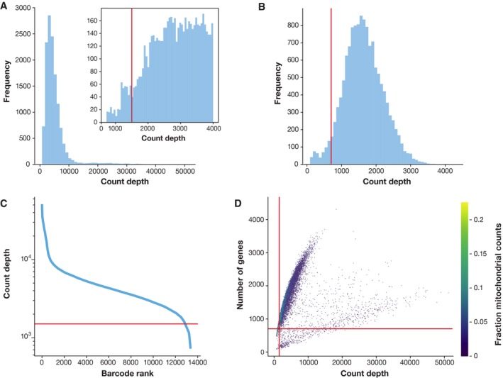
This is an example of thresholding based on the quality control covariates. The red lines represent the borders at which data points that were eliminated from the dataset (Image credits and further reading)

Data Correction

Data correction? Wasn't that normalization? Yes you are correct, but normalization alone is not enough to correct for several more complex errors. A process called regression which involves fitting data points to a line or curve. Then, marking variables that are not within a certain range of this line as outliers to be corrected. One biological factor that is sometimes regressed out is the effect of the cell cycle. At certain stages of the cell cycle, the transcriptome can widely differ which may mask other biological signals which are of more interest. Therefore, cell cycles effects are regressed out in certain studies. Similarly, count effects are sometimes regressed out as well. There are often lingering count effects despite efforts in normalization to get rid of them. This can also be dealt with by using more powerful normalization techniques. However, a general rule is that the more powerful a technique in statistics, the more likely it is to overfit the data which can be damaging to further analysis. Therefore, researchers are often cautious when using non-linear normalization algorithms.
Batch effects are also dealt with at this stage. Batch effects can happen when cells are harvested or processed at different times, when they are put on different plates, or several other experimental factors. A lot of batch effects can be mitigated with good experimental design, but alas, it looks like the role of correcting them has been placed onto the shoulders of the bioinformatician until better practices can be adopted. Batch effects can be dealt with via linear models which evaluate the contribution the batch has to its data and canceling it out, of course, this is easier said than done.
Expression recovery is a form of imputation done in biological data. Drop out events often leave behind 0s or very low expression values. Expression recovery seeks to replace these 0s with accurate expression values via machine learning algorithms. Though often times expression recovery can over correct for the noise in the data or under correct for it.
Another process done around this time is data integration. It is the process of combining data sets from different experiments or modalities in order to increase the amount of data for analysis. Though, It is so complicated that it deserves its own blog post.
After data correction, our data is finally, well, corrected. I hope you can see why biological data is some of the messiest, hard-to-work-with data out there. From batch effects, to doublets, to the stochastic nature of cells. Bioinformaticians have to put data through a washing machine before it can be used for complex tasks. The following steps of data processing are focused on simplifying the data so that it is easier to process in analysis.

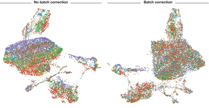
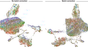
As you can see, without batch correction, each batch of data is separated due to batch effects. (Image credits and further reading)

Feature Selection and Dimensionality Reduction

First lets define some key terminology, in each barcode each gene is a feature and the number of genes together is the dimensionality. Imagine you had a Pokémon card. In the little blurb under the image it lists some basic stats, I don't blame you if you have never seen it. The blurb has the weight, size, the type of Pokémon, and the number of it in the Pokédex. Each of these stats is a feature and the total number would be the dimensionality. In this case it is a four dimensional datapoint or vector (a collection of features in the form of numbers--although some of these stats would have to be converted to numbers for the datapoint to be represented as a vector).
Researchers often narrow the number of features in the data to just 1000 - 4000 important genes that capture most of the variability or pattern in the data. These genes are called HVGs, highly variable genes. The effect of this process is that the data is much more concise and easier to work with. This is called feature selection.
However, often times we want to visualize the data. This can only happen when it is in two or three dimensions, not four thousand! More complex methods that reduce the dimensions of the data are needed. PCA finds components which are vectors of the data that maximize the variance of the data. These components can be used to represent the data in fewer dimensions. However, every time a dimension is reduced, part of the variance of the data is lost. Non-linear methods can be used to reduce the dimensions of the data while preserving more of the variance than PCA. In fact, special dimensionality reduction methods, which are often non-linear, are used for visualization due to the need to summarize the data in very few dimensions.
Generally, summarization methods are applied to the data following feature selection as the manifold of biological data is expressed in much fewer dimensions than the amount of genes. The manifold is simply the shape of the data. Imagine a bend piece of paper or cloth, you can flatten it out while keeping the general structure of the material the same. Similarly, the biological data can be flattened to much lower dimensions due to its inherent structure. Isn't that pretty cool!

Conclusion

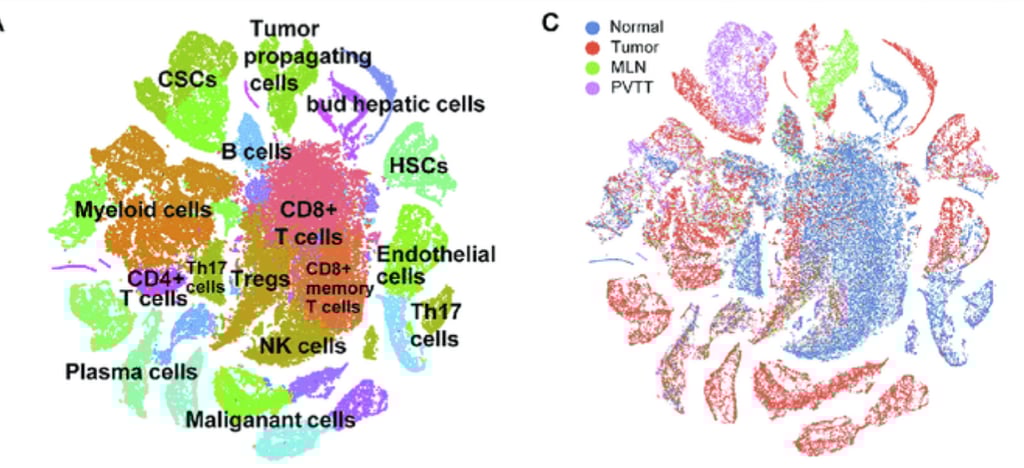
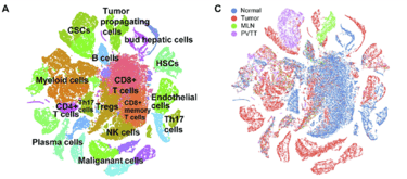
This image shows clustering, which is a process in analysis that highlights the distinct regions of cells represented in the data. It was possible only after a long arduous process of refining and cleaning the data procured from the laboratory. It represents the cumulation of several algorithms being applied to the data in order to correct for errors in sequencing, transcription, cell sorting, and countless other things. Personally, I have a new found appreciation for the work of bioinformaticians and statistics. I also have a newfound fear of single cell data. Perhaps, the complexity of such data is a result of the inherent design and structure of biological systems. Wait until we invent 20,000 dimensional glasses so that we can finally visualize raw data!

(Image credits and further reading)

Special thanks to this research paper which made my life, a LOT easier while researching for this article